Clustering

import numpy as np
import pandas as pd
import matplotlib.pyplot as plt
from sklearn.datasets import make_blobs

데이터셋 생성

sklearn패키지의 make_blobsmethod를 통해서 데이터 셋을 생성한다.

# 데이터 생성
X, y = make_blobs(n_samples = 500 , n_features = 2, centers = 4, cluster_std=1.5 , random_state =97 )

# 데이터프레임으로 재구성
target = pd.DataFrame(y)
target.columns=['Target']

data = pd.DataFrame(X)
data.columns = ['Attri_1','Attri_2']

df = pd.concat([data,target],axis=1)
df

	Attri_1	Attri_2	Target
0	-2.634632	-2.250270	1
1	4.532675	-6.285143	2
2	9.182722	8.908761	3
3	8.472858	10.529204	0
4	5.582174	7.721625	0
...	...	...	...
495	9.352046	8.388088	3
496	8.149692	9.503454	3
497	-0.084687	-4.759452	1
498	5.676850	10.491732	0
499	8.457310	-3.120653	2

500 rows × 3 columns

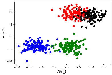
# Data Plot
col = pd.Series(df['Target']).map({0:'red',1:'blue',2:'green',3:'black'})
plt.scatter(df['Attri_1'],df['Attri_2'],c=col)
plt.xlabel('Attri_1')
plt.ylabel('Attri_2')
plt.show()

png

# 사용할 속성 추출
feature = df[['Attri_1','Attri_2']]
feature.tail()

	Attri_1	Attri_2
495	9.352046	8.388088
496	8.149692	9.503454
497	-0.084687	-4.759452
498	5.676850	10.491732
499	8.457310	-3.120653

K-means Clustering

실습 파일에서와 마찬가지로, 클러스터링과 시각화 및 Elbow rule을 통한 검증을 진행합니다.

시각화 진행 시, plot에 클러스터 중심의 위치를 나타냅니다.

# K-means Clustering Algorithm
from sklearn.cluster import KMeans

# 모델 생성
kmeans = KMeans(n_clusters=4,max_iter=50)
# 모델 피팅
kmeans.fit(feature)

KMeans(max_iter=50, n_clusters=4)

# 피팅 결과 생성된 클러스터 라벨
kmeans.labels_

# 각 클러스터의 클러스터 센트로이드
kmeans.cluster_centers_

array([[ 6.48539263,  9.4436022 ],
       [ 5.74813556, -4.2879631 ],
       [-1.00013483, -4.10072491],
       [ 9.9020639 ,  8.32587273]])

# SSE (Sum of Squared Distances of samples to their closest cluster center)
kmeans.inertia_

2005.1793171587194

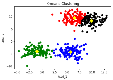
# Clustered result
col_cluster = pd.Series(kmeans.labels_).map({0:'red',1:'blue',2:'green',3:'black'})
f1 = plt.figure(1)
plt.scatter(df['Attri_1'],df['Attri_2'],c=col_cluster)
plt.scatter(kmeans.cluster_centers_[:,0],kmeans.cluster_centers_[:,1], c='yellow', s=70, marker='D') # cluster centroids
plt.title('Kmeans Clustering')
plt.xlabel('Attri_1')
plt.ylabel('Attri_2')


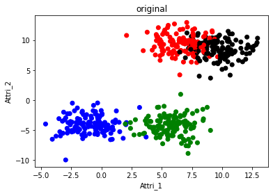
# Original data
f2 = plt.figure(2)
plt.scatter(df['Attri_1'],df['Attri_2'],c=col)
plt.xlabel('Attri_1')
plt.ylabel('Attri_2')
plt.title('original')
plt.show()

png

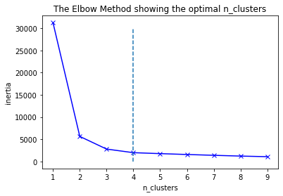
num_clusters = range(1,10)
inertias = []

for num in num_clusters:
    kmeanModel = KMeans(n_clusters=num)
    kmeanModel.fit(feature)
    inertias.append(kmeanModel.inertia_)
plt.plot(num_clusters, inertias, 'bx-')
plt.xlabel('n_clusters')
plt.ylabel('inertia')
plt.title('The Elbow Method showing the optimal n_clusters')
plt.plot(np.linspace(4,4,6),np.linspace(-1,30000,6),'--')
plt.show()

png

DBSCAN

실습 파일에서와 마찬가지로, 클러스터링과 시각화를 진행합니다.

# DBSCAN clustering algorithm
from sklearn.cluster import DBSCAN

# 모델 생성
dbscan = DBSCAN(eps=0.7, min_samples=5)
# 모델 피팅
dbscan.fit(feature)

DBSCAN(eps=0.7)

set(dbscan.labels_)

{-1, 0, 1, 2, 3, 4}

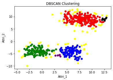
# Clustered result
col_cluster_1 = pd.Series(dbscan.labels_).map({-1:'yellow',0:'red',1:'blue',2:'green',3:'black',4:'purple'})
f1 = plt.figure(1)
plt.scatter(df['Attri_1'],df['Attri_2'],c=col_cluster_1)
plt.title('DBSCAN Clustering')
plt.xlabel('Attri_1')
plt.ylabel('Attri_2')


# Original data
f2 = plt.figure(2)
plt.scatter(df['Attri_1'],df['Attri_2'],c=col)
plt.xlabel('Attri_1')
plt.ylabel('Attri_2')
plt.title('original')
plt.show()

png

AGNES

실습 파일에서와 마찬가지로, 두 가지 클래스를 모두 이용하여 클러스터링과 시각화를 진행합니다.

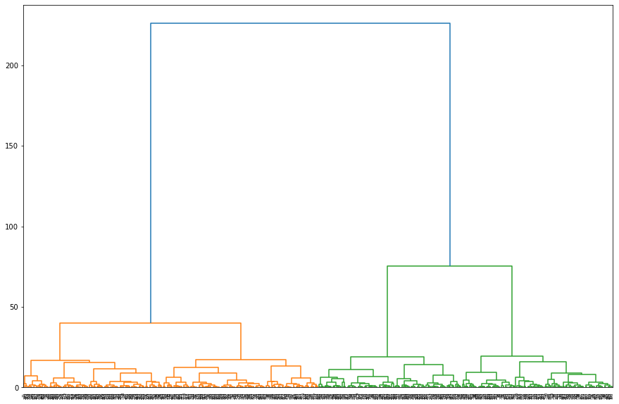
후자의 경우 덴드로그램도 그려주세요!
linkage의 경우 ward 아니라 세션에서 다루었던 다른 거리 측정방식을 사용해도 좋습니다!

sklearn.cluster.AgglomerativeClustering

from sklearn.cluster import AgglomerativeClustering

# 모델 생성
agnes = AgglomerativeClustering(n_clusters=4)
# 모델 피팅
agnes.fit(feature)

AgglomerativeClustering(n_clusters=4)

# 피팅 결과 생성된 클러스터 라벨
agnes.labels_

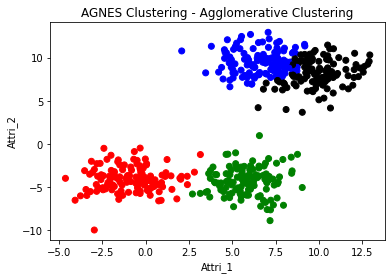
# Clustered result
col_cluster_2 = pd.Series(agnes.labels_).map({0:'red',1:'blue',2:'green',3:'black'})
f1 = plt.figure(1)
plt.scatter(df['Attri_1'],df['Attri_2'],c=col_cluster_2)
plt.title('AGNES Clustering - Agglomerative Clustering')
plt.xlabel('Attri_1')
plt.ylabel('Attri_2')


# Original data
f2 = plt.figure(2)
plt.scatter(df['Attri_1'],df['Attri_2'],c=col)
plt.xlabel('Attri_1')
plt.ylabel('Attri_2')
plt.title('original')
plt.show()

png

scipy.cluster.hierarchy

from scipy.cluster.hierarchy import linkage, cut_tree
# from scipy.cluster.hierarchy import ward, cut_tree

linkage_array = linkage(feature, method='ward')
# linkage_array = ward(feature)

linkage_array

array([[7.40000000e+01, 2.76000000e+02, 1.25463773e-03, 2.00000000e+00],
       [3.08000000e+02, 3.40000000e+02, 1.73685772e-02, 2.00000000e+00],
       [1.21000000e+02, 4.16000000e+02, 2.02554219e-02, 2.00000000e+00],
       ...,
       [9.92000000e+02, 9.93000000e+02, 3.97321894e+01, 2.50000000e+02],
       [9.94000000e+02, 9.95000000e+02, 7.53068455e+01, 2.50000000e+02],
       [9.96000000e+02, 9.97000000e+02, 2.26161762e+02, 5.00000000e+02]])

label_cluster = cut_tree(linkage_array, n_clusters=4)
label_cluster = [lab[0] for lab in label_cluster]

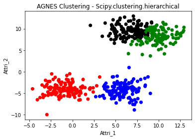
# Clustered result
col_cluster_2 = pd.Series(label_cluster).map({0:'red',1:'blue',2:'green',3:'black'})
f1 = plt.figure(1)
plt.scatter(df['Attri_1'],df['Attri_2'],c=col_cluster_2)
plt.title('AGNES Clustering - Scipy.clustering.hierarchical')
plt.xlabel('Attri_1')
plt.ylabel('Attri_2')


# Original data
f2 = plt.figure(2)
plt.scatter(df['Attri_1'],df['Attri_2'],c=col)
plt.xlabel('Attri_1')
plt.ylabel('Attri_2')
plt.title('original')
plt.show()

png

from scipy.cluster.hierarchy import dendrogram

plt.figure(figsize=(15,10))
fig = dendrogram(linkage_array)

png

클러스터링 결과 비교

generate된 데이터가 어떠한 클러스터링 알고리즘에서 가장 분류가 잘 되었는지, 어떤 알고리즘에서 가장 분류가 안 되었는지 보고, 그 이유를 추측해서 간단하게 써주세요!

# Data Plot
col_cluster = pd.Series(kmeans.labels_).map({0:'red',1:'blue',2:'green',3:'black'})
f1 = plt.figure(1)
plt.scatter(df['Attri_1'],df['Attri_2'],c=col_cluster)
plt.scatter(kmeans.cluster_centers_[:,0],kmeans.cluster_centers_[:,1], c='yellow', s=70, marker='D') # cluster centroids
plt.title('Kmeans Clustering')
plt.xlabel('Attri_1')
plt.ylabel('Attri_2')


# Clustered result
col_cluster_1 = pd.Series(dbscan.labels_).map({-1:'yellow',0:'red',1:'blue',2:'green',3:'black',4:'purple'})
f1 = plt.figure(2)
plt.scatter(df['Attri_1'],df['Attri_2'],c=col_cluster_1)
plt.title('DBSCAN Clustering')
plt.xlabel('Attri_1')
plt.ylabel('Attri_2')



# Clustered result
col_cluster_2 = pd.Series(label_cluster).map({0:'red',1:'blue',2:'green',3:'black'})
f1 = plt.figure(3)
plt.scatter(df['Attri_1'],df['Attri_2'],c=col_cluster_2)
plt.title('AGNES Clustering - Scipy.clustering.hierarchical')
plt.xlabel('Attri_1')
plt.ylabel('Attri_2')


# Original data
f2 = plt.figure(4)
plt.scatter(df['Attri_1'],df['Attri_2'],c=col)
plt.xlabel('Attri_1')
plt.ylabel('Attri_2')
plt.title('original')
plt.show()

png

결론

AGNES가 가장 분류가 잘 되었고 DBSCAN이 가장 분류가 안 되었다.

AGNES

AGNES의 경우 각각의 성분들이 존재하였을때 가장 가까운 것들을 천천히 합쳐 나가는 방식이다. ward를 사용하게 된다면 두 집단을 합쳤을 때 centroid가 얼마나 바뀌는가이다. 가장 적게 바뀐다면 두 가지를 합치는 방식이다.
- K-means의 경우 centroid가 그대로인 상태로 다른 점들을 포함할 것인가 아닌가를 따지는 것 이기 때문에 약간은 다르다고 할 수 있다.
주어진 dataset을 관찰하면, 하단에 있는 두 가지 부류는 K-mean과 AGENS가 거의 동일하게 나누었지만, 상단에 있는 두 가지 부류는 AGNES가 더 잘 분류를 했다는 것을 확인할 수 있는데, 그 이유는 다음과 같다.
- Clustering은 전쟁과 비슷하다. 도시국가들이 싸워서 합병을 하는 것인지 혹은 큰나라 두 개가 수 많은 성들을 나누어 먹는 것인지의 차이라고 생각하면 편할 것 같다.
- K-means의 경우 후자라고 할 수 있다. centroid에 가까우면 먹고 아니면 주는 형태를 취하기 때문에 위의 첫 번째 그림처럼 국경이 완벽하게 갈린 것이라고 볼 수 있다.
- AGENS의 경우 전자라고 할 수 있다. 도시국가들이 생겨나고 가장 가까운 도시국가들끼리 싸워서 이기는 나라가 점차 성장한다고 볼 수 있다. 이렇게 세력다툼을 하다가 마지막에 큰 나라 두 개가 생기는 것인데, 이 과정속에서 국경이 일직선으로 유지될 수가 없을 것이다.
- 그런데 original을 보면 black과 red가 서로 침투되어있는 것을 확인할 수 있다.
- $\therefore$ K-means보다 AGNES의 경우 상대적으로 국경이 곡선인 AGNES가 더 적합했다고 말할 수 있겠다.

DBSCAN

DBSCAN은 commment를 남길 것이 없을 정도로 해당 데이터 셋에 대해서 최악인 이유가 명확하다.
- 상위 두 집단은 어떠한 pattern을 띠고 있지 않다. DBSCAN은 특정한 pattern을 띨 때 유용하게 쓰일 수 있는데, 오히려 겹쳐져 있는 형태를 띤다. 따라서 애초에 절대 제대로 Clustering이 될 수 없다.

이 문서는 DSL과제 template을 그래도 가져왔음.

DSL Clustering

DSL lecture on 16SEP20

Clustering

데이터셋 생성

K-means Clustering

DBSCAN

AGNES

sklearn.cluster.AgglomerativeClustering

scipy.cluster.hierarchy

클러스터링 결과 비교

결론

AGNES

DBSCAN